Understand multiple signals
User Equity observed series Stress observed series
How do they relate?
Assistant Stress leads each equity drawdown.
%20{%20.material%20{%20display:%20none;%20}%20.base%20{%20fill:%20%23fff;%20}%20}%20%3c/style%3e%3cdefs%3e%3cpath%20id='ribbon'%20d='M153%20120%20L252%2030%20Q265%2016%20281%2033%20L439%20191%20Q460%20211%20443%20230%20L394%20273%20L291%20169%20Q253%20130%20232%20123%20Q205%20113%20181%20124%20L168%20133%20Q158%20138%20153%20130%20Q150%20125%20153%20120%20Z%20M48%20273%20L176%20147%20Q205%20120%20234%20144%20L267%20176%20L96%20355%20L48%20308%20Q30%20290%2048%20273%20Z%20M290%20393%20L470%20216%20L512%20259%20Q530%20275%20514%20297%20L387%20424%20Q355%20454%20328%20425%20Z%20M122%20340%20L169%20293%20L297%20422%20Q335%20461%20372%20441%20L378%20438%20Q395%20435%20388%20449%20L300%20524%20Q285%20540%20270%20524%20L123%20373%20Q108%20358%20122%20340%20Z'/%3e%3cclipPath%20id='weave'%3e%3cuse%20href='%23ribbon'/%3e%3c/clipPath%3e%3c!--%20Rounded%20corners%20keep%20material%20moving%20smoothly%20through%20each%20fold.%20--%3e%3cpath%20id='track'%20pathLength='1000'%20d='M296%20106%20L454%20264%20Q470%20280%20454%20296%20L296%20454%20Q280%20470%20264%20454%20L106%20296%20Q90%20280%20106%20264%20L264%20106%20Q280%2090%20296%20106%20Z'/%3e%3cfilter%20id='soft'%20x='-50%25'%20y='-50%25'%20width='200%25'%20height='200%25'%3e%3cfeGaussianBlur%20stdDeviation='22'/%3e%3c/filter%3e%3cfilter%20id='fold'%20x='-50%25'%20y='-50%25'%20width='200%25'%20height='200%25'%3e%3cfeGaussianBlur%20stdDeviation='9'/%3e%3c/filter%3e%3c/defs%3e%3cuse%20class='base'%20href='%23ribbon'%20fill='%23AEB9BE'/%3e%3c!--%20Clip%20after%20blurring,%20so%20the%20original%20over/under%20cuts%20remain%20crisp.%20--%3e%3cg%20class='material'%20clip-path='url(%23weave)'%20fill='none'%20stroke-width='200'%20stroke-linejoin='round'%3e%3cg%20filter='url(%23soft)'%20stroke='%23FFF'%3e%3cuse%20class='flow'%20href='%23track'%20stroke-dasharray='340%20660'/%3e%3cuse%20class='flow%20second'%20href='%23track'%20stroke-dasharray='340%20660'%20opacity='.72'/%3e%3c/g%3e%3cuse%20class='flow%20crease'%20href='%23track'%20stroke='%2323343D'%20stroke-dasharray='24%20476'%20opacity='.3'%20filter='url(%23fold)'/%3e%3c/g%3e%3c/svg%3e) TimeBraid:Unifying Time Series and Language for Understanding and Forecasting
TimeBraid:Unifying Time Series and Language for Understanding and ForecastingUnderstand, forecast, and shape time series with language.
The idea
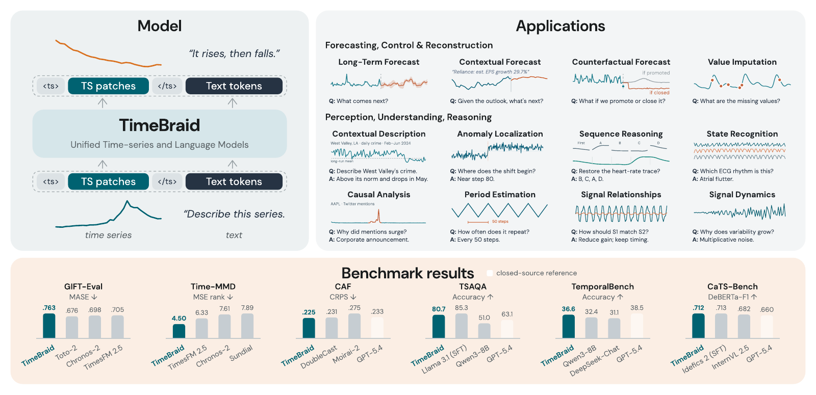
TimeBraid brings pretrained language and time-series models into one framework. It connects language knowledge and reasoning with continuous-signal perception and forecasting, so the same model can understand a signal, explain it in words, and generate what comes next.
Method
Language tokens and numerical time-series patches pass through their pretrained backbones. Interleaved global residual attention connects the streams at multiple depths: each token can draw on earlier context from both modalities, and the updates return to each backbone through residual connections.
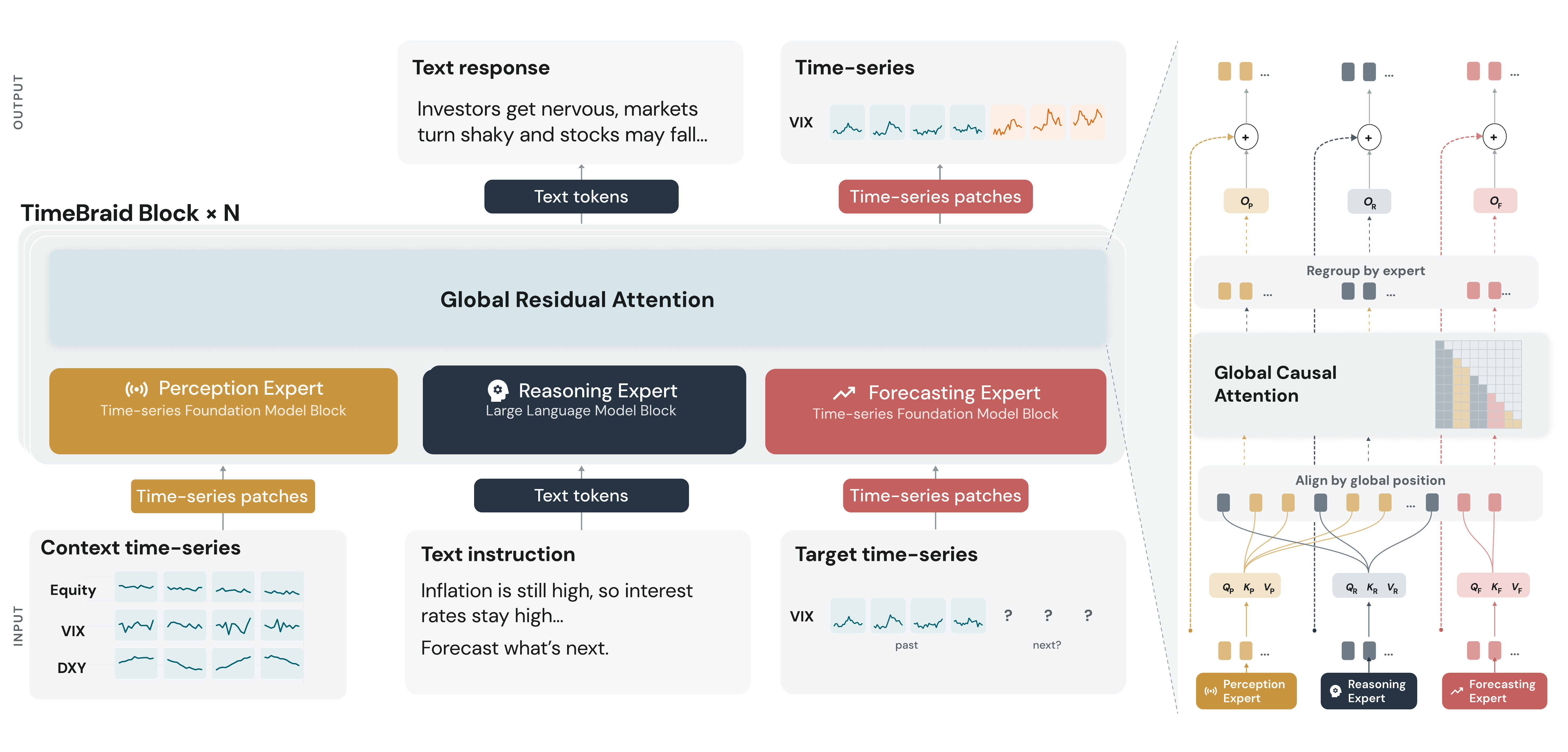
Encodes observed time-series segments and the structure within them.
Processes instructions and context, and generates language responses.
Generates future time-series segments from numerical and textual context.
TimeBraid treats a task as an ordered sequence of text and time-series segments. Each output draws on the segments before it. Multiple variables enter as separate signals, each bound to a <ts></ts> marker. Text becomes language tokens; signals become patches of 32 continuous values.
Understand multiple signals
User Equity observed series Stress observed series
How do they relate?
Assistant Stress leads each equity drawdown.
Generate a conditioned forecast
User CPU load observed series
A deployment just shipped. Forecast the next 96 hours.
Assistant future numerical patches
Illustrative prompt structures from Section 3.2. Context time-series segments carry their length, mean and standard deviation. Numerical payloads remain separate from the text transcript.
The forecasting expert predicts numerical patches autoregressively, with a central trajectory and nine quantiles for uncertainty. Text responses use next-token prediction. The two output types learn together through separate language and forecasting losses.
Training recipe
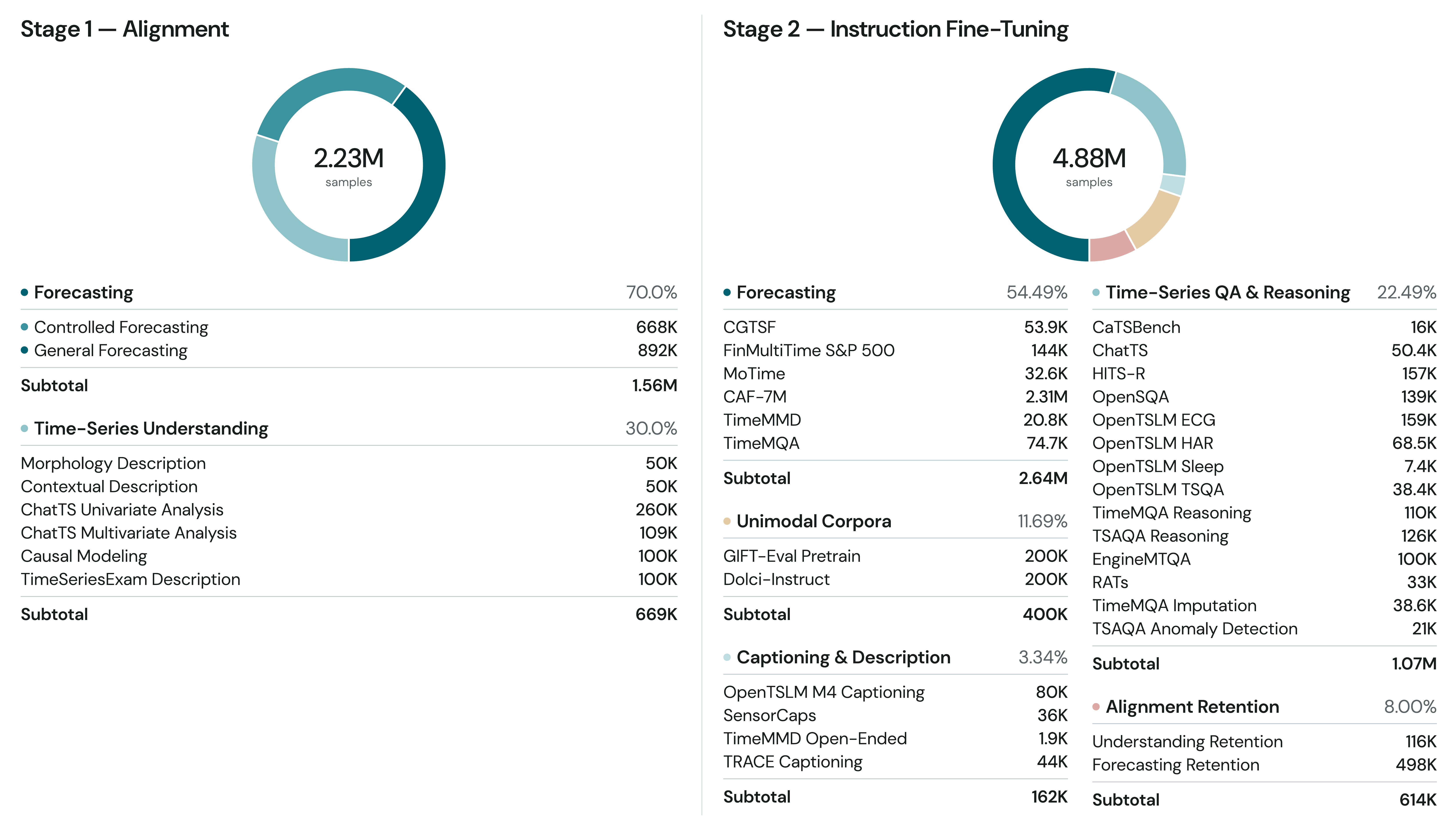
A two-stage curriculum connects temporal structure with language, then extends that foundation to instruction following and real-world tasks.
Stage 1 · Alignment
Descriptions, analysis and forecasting examples teach the model how signals relate to language and how different conditions lead to different futures.
30% understanding · 70% forecasting
Stage 2 · Instruction tuning
A diverse mixture covers forecasting, question answering, reasoning and captioning across energy, climate, healthcare, finance, sensing and industrial monitoring.
Domain tasks · Unimodal data · Alignment retention
Understanding pairs combine morphology and context-rich captions, attribute-first synthetic signals, structural causal models and programmable questions. Forecast-control pairs give one history several possible futures, each described by its own condition.
Forecast annotations are created with access to the future and can describe the target interval; future numerical values are excluded from the model input. These pairs teach conditional generation under stated scenarios.
Paper benchmarks
Aggregate results under the paper’s evaluation protocols, across temporal understanding, contextual forecasting and language.
Understand patterns, anomalies and temporal relationships.
Scroll horizontally for all metrics
| Model | Overall ↑Accuracy (%) |
|---|---|
| TimeBraid-2.5B | 78.31 |
| TimeBraid-6.7B | 80.65 |
| LLaMA3.1-8B (SFT) | 85.26 |
| Closed-source reference · not ranked | |
| Gemini-2.5-Flash | 65.08 |
| GPT-5.4 | 63.10 |
Official test-set accuracy. The SFT baseline is finetuned on TSAQA training data.
Reason about patterns, noise, anomalies, similarity and causality.
Scroll horizontally for all metrics
| Model | Overall ↑Accuracy (%) |
|---|---|
| TimeBraid-2.5B | 60.05 |
| TimeBraid-6.7B | 63.14 |
| TS-Reasoner-7B | 54.26 |
| Closed-source reference · not ranked | |
| GPT-4.1 (vision) | 67.89 |
| GPT-5.4 | 67.83 |
Overall multiple-choice accuracy. GPT-4.1 uses the vision input setting.
Describe time series with accurate language and numbers.
Scroll horizontally for all metrics
| Model | DeBERTa F1 ↑Score [0, 1] | SimCSE ↑Score [0, 1] | Numeric Fidelity ↑Score [0, 1] |
|---|---|---|---|
| TimeBraid-2.5B | 0.708 | 0.885 | 0.670 |
| TimeBraid-6.7B | 0.712 | 0.886 | 0.684 |
| Idefics 2 (finetuned) | 0.713 | 0.885 | 0.748 |
| Qwen3-8B | 0.670 | 0.865 | 0.678 |
| LLaMA3.1-8B-Instruct | 0.667 | 0.859 | 0.697 |
| Closed-source reference · not ranked | |||
| Gemini 2.5 Flash | 0.694 | 0.887 | 0.802 |
Human-rewritten split. The text-only baselines receive series and metadata without plots; Idefics 2 is finetuned on CaTS-Bench.
Connect temporal perception, prediction and contextual reasoning.
Scroll horizontally for all metrics
| Model | Overall ↑Macro accuracy (%) |
|---|---|
| TimeBraid-2.5B | 35.74 |
| TimeBraid-6.7B | 36.58 |
| Closed-source reference · not ranked | |
| GPT-5.4 | 38.50 |
| GPT-4.1 | 36.91 |
| Gemini-2.5-Flash | 34.61 |
Macro accuracy over 16 tasks in four domains. Forecasting errors and task breakdowns are in the full results.
Use aligned text to forecast across nine real-world domains.
Scroll horizontally for all metrics
| Model | MSE rank ↓Mean rank | MAE rank ↓Mean rank |
|---|---|---|
| TimeBraid-2.5B | 5.11 | 5.11 |
| TimeBraid-6.7B | 4.50 | 4.78 |
| TimesFM2.5 | 6.33 | 5.44 |
| Chronos-2 | 7.61 | 6.50 |
| MIGAS-1.5 | 8.06 | 6.56 |
Published ranks over the full comparison set; four horizons per domain. These models use 128-step histories.
Forecast solar power, electricity usage and traffic with context.
Scroll horizontally for all metrics
| Model | Macro MSE ↓ | Macro MAE ↓ |
|---|---|---|
| TimeBraid-2.5B | 0.415 | 0.338 |
| TimeBraid-6.7B | 0.413 | 0.338 |
| GPT4MTS | 0.481 | 0.397 |
| Time-LLM | 0.482 | 0.409 |
| Chronos-2 | 0.531 | 0.363 |
Standardized errors averaged over three datasets and four history lengths.
Improve probabilistic forecasts with informative text.
Scroll horizontally for all metrics
| Model | Normalized CRPS ↓Mean ± s.e. |
|---|---|
| TimeBraid-2.5B | 0.235 ± 0.012 |
| TimeBraid-6.7B | 0.225 ± 0.012 |
| DoubleCast | 0.231 ± 0.001 |
| Moirai-2 | 0.275 ± 0.014 |
| Closed-source reference · not ranked | |
| GPT-5.4 | 0.233 ± 0.011 |
Pooled test-set mean ± standard error. DoubleCast is reported by the CAF-7M paper.
Generate different futures for the same history and new conditions.
Scroll horizontally for all metrics
| Model | MSE ↓ | Top-1 ↑Accuracy (%) |
|---|---|---|
| TimeBraid-2.5B | 6.972 | 40.67 |
| TimeBraid-6.7B | 6.232 | 43.33 |
| Moirai-2 | 8.425 | 33.33 |
| Closed-source reference · not ranked | ||
| GPT-5.4 | 5.188 | 51.33 |
| GPT-4o | 5.447 | 60.00 |
History-normalized MSE and correct-sibling retrieval on 150 windows; chance Top-1 is 33.33%.
Forecast with background knowledge and future context.
Scroll horizontally for all metrics
| Model | RCRPS ↓Mean ± s.e. |
|---|---|
| TimeBraid-2.5B | 0.289 ± 0.002 |
| TimeBraid-6.7B | 0.294 ± 0.002 |
| Moirai-2* | 0.288 ± 0.002 |
| Closed-source reference · not ranked | |
| Gemini-2.5-Flash | 0.110 ± 0.002 |
| GPT-5.4 | 0.145 ± 0.000 |
Task-weighted RCRPS, mean ± standard error. *Without natural-language context.
Point and probabilistic forecasting across 97 configurations.
Scroll horizontally for all metrics
| Model | MASE ↓ | CRPS ↓ |
|---|---|---|
| TimeBraid-2.5B | 0.763 | 0.546 |
| Toto-2.0-FnF | 0.676 | 0.463 |
| Chronos-2 | 0.698 | 0.485 |
| TimesFM 2.5 | 0.705 | 0.490 |
| Seasonal Naive | 1.000 | 1.000 |
Geometric means normalized against Seasonal Naive. TimeBraid-2.5B uses 2,880 history steps.
Long-horizon forecasting on ETTm1, ETTm2, ETTh1, ETTh2 and Weather.
Scroll horizontally for all metrics
| Model | MSE rank ↓Mean rank | MAE rank ↓Mean rank |
|---|---|---|
| TimeBraid-2.5B | 2.48 | 3.45 |
| Sundial-Large | 2.23 | 4.15 |
| Chronos-2 | 2.80 | 1.20 |
| TimesFM-2.5 | 3.83 | 2.25 |
| TimeMixer | 5.67 | 5.80 |
Published ranks across 20 settings. TimeMixer is trained per dataset; the other displayed models are zero-shot.
Track general language ability through TimeBraid-2.5B training.
Scroll horizontally for all metrics
| Training stage | Accuracy ↑Five-shot MMLU (%) |
|---|---|
| Base (Qwen3-1.7B language tower) | 60.30 |
| Align | 40.88 |
| SFT | 50.68 |
Five-shot MMLU with the standard training recipe. SFT recovers much of the alignment-stage loss.
Selected models and headline metrics from each benchmark. TimeBraid model sizes count all parameters. Bold marks the best displayed value. Following the paper, closed-source commercial models are listed as reference points below the divider and stay outside the ranking. ± denotes standard error.
Evaluation examples are held out at the split level. TemporalBench MCQ, CiK, and ETT/Weather are outside the training mixture. TSAQA, CaTS, TimeMMD, CGTSF and CAF contribute training-split data.
TimeSeriesExam and Ctrl-F share their data-generating process with independently generated alignment examples. Part of GIFT-Eval’s training split provides seed data for generation. These settings test different forms of generalization.
Ablations & findings
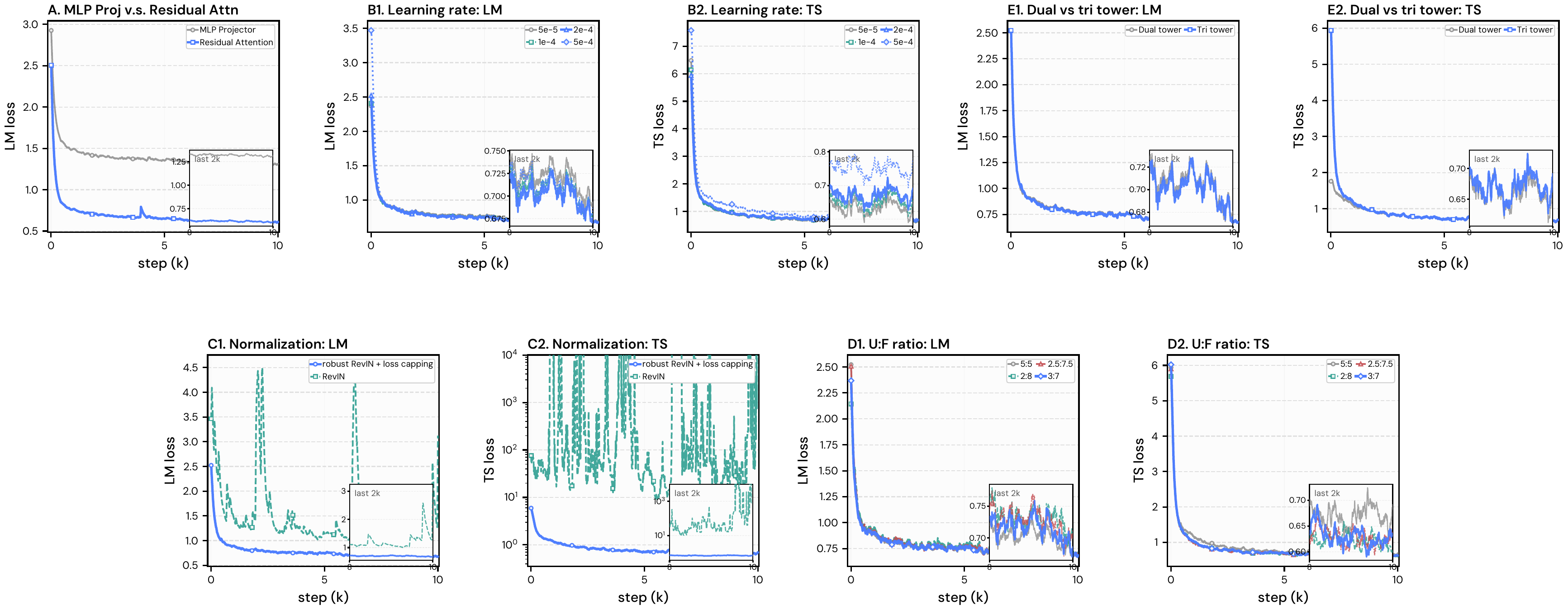
Six research questions test the interface, architecture, optimization, curriculum and use of text. The results explain the choices behind TimeBraid.
RQ1 · Interaction space
Residual attention reaches substantially lower language loss than projecting time-series features directly into the language space with an MLP connector.
RQ2 · Expert separation
Separate perception and forecasting towers yield nearly identical training-loss curves to a shared time-series tower in the tested alignment runs.
RQ3 · Optimization stability
Nonstationary targets can produce large forecasting losses that also disrupt language learning. Robust normalization compresses extreme values; response-level loss capping limits their contribution.
RQ4 · Modality balance
The 30:70 understanding-to-forecasting mixture improves forecasting loss over an even split without worsening language loss. The final recipe weights the time-series loss by 0.5.
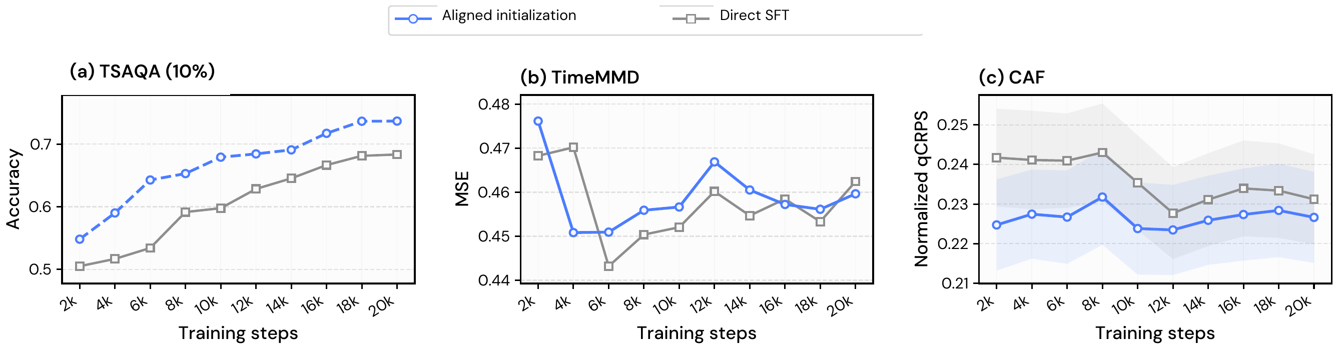
RQ5 · Alignment before instruction tuning
Aligned initialization stays ahead on TSAQA and CAF throughout instruction tuning. TimeMMD finishes at similar error with either initialization, showing that the benefit depends on the task and its use of text.
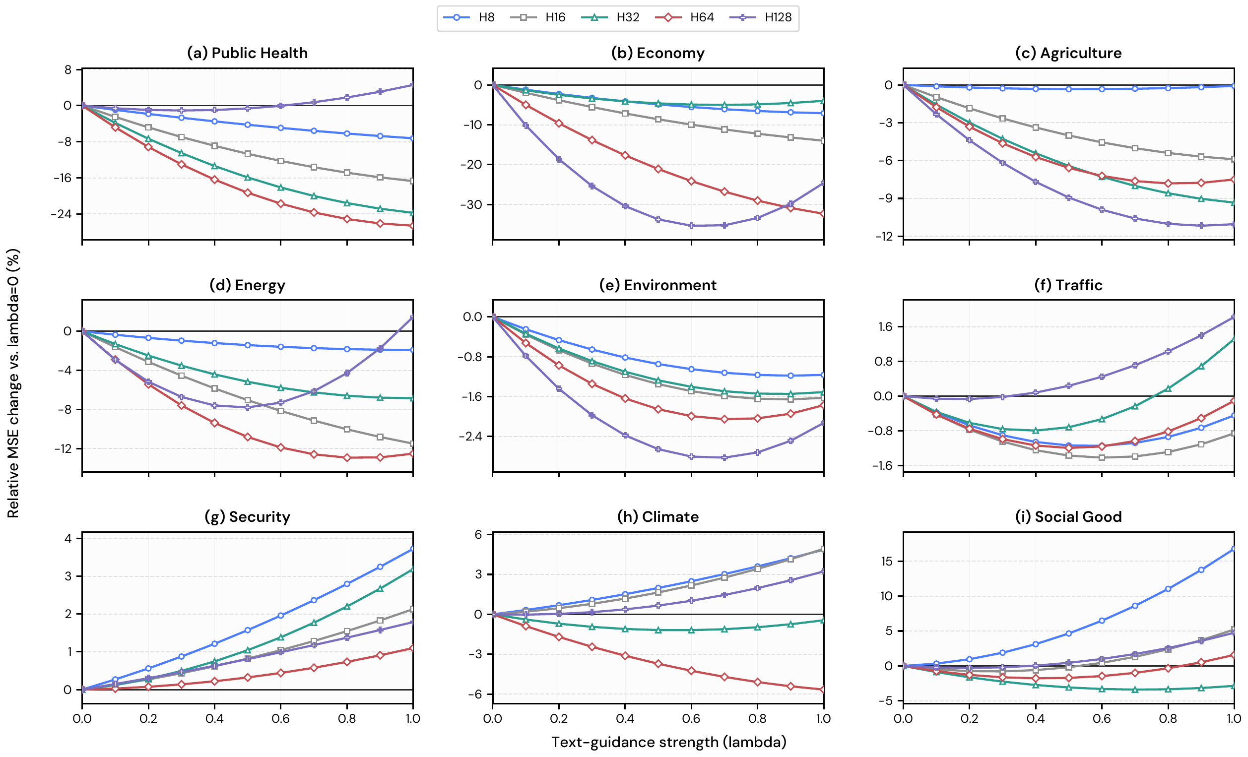
RQ6 · Text strength at inference
Run the same model with history alone and with history plus text, then mix the two point forecasts. The weight λ moves from the history-only prediction at 0 to the fully conditioned prediction at 1.
In the TimeMMD sweep, the effect of text varies with the domain and history length. Security favors history alone; Climate and Social Good change with history length. The TimeMMD comparison uses one validation-selected λ = 0.3 across all domains.
Numerical detail. Patch compression can lose exact local values and make long, high-frequency or noisy waveforms difficult to read. CaTS captions still miss numerical details compared with stronger captioning baselines.
Forecast control. Abrupt changes that contradict the history are followed less reliably. Complex or weakly related text remains difficult to translate into numerical consequences.
Training coverage. The recipe moves from alignment directly to instruction tuning. Broader interleaved pretraining data and better language-retention mixtures remain open directions.
Explore TimeBraid
Ask about temporal patterns, reason across signals, or change the conditions of a forecast. Explore language and time series through the same model.
Selected field cases · 2024–2026
Freshly collected public series across markets, the macro economy, air quality, weather, power grids and the web. These selected cases show TimeBraid outperforming the baselines displayed here; see the paper benchmarks for aggregate results.
TimeBraid sees nothing but each series’ own past values: no name, no unit, no dates. The baselines receive exactly the same numbers.
Equities · US equities
Forecast Jun 2 – Aug 31, 2026 · next 63 trading days
Input: 512 past observations only
Series: Yahoo Finance chart API ↗
Crypto · Global crypto markets
Forecast Jun 21 – Sep 12, 2026 · next 84 days
Input: 672 past observations only
Series: Yahoo Finance chart API ↗
Rates · United States
Forecast Jul 23 – Aug 31, 2026 · next 28 days
Input: 672 past observations only
Rivers · Richmond, Virginia
Forecast Aug 7 – Sep 3, 2026 · next 28 days
Input: 672 past observations only
Air quality · Los Angeles, California
Forecast Jul 11 – Sep 4, 2026 · next 56 days
Input: 672 past observations only
Series: Open-Meteo Air Quality API (CAMS global/European reanalysis) ↗
Weather · Helsinki, Finland
Forecast Jun 21 – Sep 12, 2026 · next 84 days
Input: 672 past observations only
Series: Open-Meteo Historical Weather API (ERA5 reanalysis) ↗
Power grid · Malmö, Sweden (zone SE4)
Forecast Jul 25 – Sep 18, 2026 · next 56 days
Input: 672 past observations only
Series: energy-charts.info API (Fraunhofer ISE), day-ahead price, CC BY 4.0 ↗
Weather · Sydney, Australia
Forecast Jun 30 – Aug 24, 2026 · next 56 days
Input: 672 past observations only
Series: Open-Meteo Historical Weather API (ERA5 reanalysis) ↗
Rivers · Romeoville, Illinois
Forecast Aug 18 – Sep 14, 2026 · next 28 days
Input: 672 past observations only
Macro · United States
Forecast Jun 11 – Sep 2, 2026 · next 84 days
Input: 672 past observations only
Dated reports enter alongside the observed series, before the forecast period begins.
Currencies · Chile
Forecast Dec 15 – Dec 23, 2025 · next 7 trading days
Input: 256 past observations and the report below
Series: Yahoo Finance chart API ↗
Air quality · Porto Velho, Brazil
Forecast Sep 10 – Sep 19, 2024 · next 10 days
Input: 365 past observations and the report below
Series: Open-Meteo air quality ↗
Equities · Oslo Stock Exchange
Forecast Nov 17 – Dec 5, 2025 · next 15 trading days
Input: 256 past observations and the report below
Series: Yahoo Finance chart API ↗
Web attention · English Wikipedia
Forecast Feb 20 – Feb 24, 2025 · next 5 days
Input: 365 past observations and the report below
Series: Wikimedia pageviews API ↗
Commodities · ICE, London
Forecast Aug 10 – Aug 28, 2026 · next 15 trading days
Input: 256 past observations and the report below
Series: Yahoo Finance chart API ↗
Commodities · COMEX, New York
Forecast Oct 8 – Oct 16, 2025 · next 7 trading days
Input: 256 past observations and the report below
Series: Yahoo Finance chart API ↗
Air quality · Castaic, California
Forecast Jan 23 – Jan 27, 2025 · next 5 days
Input: 365 past observations and the report below
Series: Open-Meteo air quality ↗
Weather · Hanoi, Vietnam
Forecast Sep 8 – Sep 12, 2024 · next 5 days
Input: 365 past observations and the report below
Series: Open-Meteo archive ↗
Weather · Đồng Hới, Vietnam
Forecast Aug 26 – Aug 30, 2025 · next 5 days
Input: 365 past observations and the report below
Series: Open-Meteo archive ↗
Weather · Brownsville, Texas
Forecast Jun 18 – Jun 22, 2026 · next 5 days
Input: 365 past observations and the report below
Series: Open-Meteo archive ↗
Real reporting is long and indirect. GPT-6 Luna rewrites each report into a short instruction (direction, timing and strength, without target values), and TimeBraid follows it. The faded line is TimeBraid’s forecast from the original report. The baselines read the original report.
Currencies · Currency markets
Forecast Jan 22 – Jan 30, 2026 · next 7 trading days
Input: 256 past observations and the report below
Series: Yahoo Finance chart API ↗
Macro · United States, weekly average
Forecast Mar 30 – Apr 13, 2026 · next 3 weeks
Input: 104 past observations and the report below
Series: FRED ↗
Macro · US equity options
Forecast Mar 2 – Mar 13, 2026 · next 10 days
Input: 365 past observations and the report below
Series: FRED ↗
Commodities · NYMEX, New York
Forecast Mar 16 – Mar 24, 2026 · next 7 trading days
Input: 256 past observations and the report below
Series: Yahoo Finance chart API ↗
Commodities · ICE, New York
Forecast Aug 4 – Aug 22, 2025 · next 15 trading days
Input: 256 past observations and the report below
Series: Yahoo Finance chart API ↗
Equities · Tel Aviv Stock Exchange
Forecast Dec 18, 2025 – Jan 12, 2026 · next 15 trading days
Input: 256 past observations and the report below
Series: Yahoo Finance chart API ↗
Equities · New York Stock Exchange
Forecast Jun 10 – Jun 18, 2026 · next 7 trading days
Input: 256 past observations and the report below
Series: Yahoo Finance chart API ↗
Currencies · Pakistan
Forecast Apr 24 – May 4, 2025 · next 7 trading days
Input: 256 past observations and the report below
Series: Yahoo Finance chart API ↗
Weather · Irish Sea, off Anglesey
Forecast Dec 8 – Dec 12, 2024 · next 5 days
Input: 365 past observations and the report below
Series: Open-Meteo archive ↗
Seismology · Mexico, magnitude 3+
Forecast Jan 3 – Jan 7, 2026 · next 5 days
Input: 365 past observations and the report below
Series: USGS Earthquake Catalog (ComCat FDSN event service) ↗
Information processing
You Language
Extract the event details from this notice as a JSON object with keys title, date, start_time, venue, and capacity.
The workshop "Build a Tiny Robot" will take place on 18 October 2026 at the Riverside Library. It starts at 14:30 and has space for 24 participants.
Use YYYY-MM-DD for the date and a number for capacity. Return only the JSON.
∿TimeBraid Language
{
  "title": "Build a Tiny Robot",
  "date": "2026-10-18",
  "start_time": "14:30",
  "venue": "Riverside Library",
  "capacity": 24
}{
"title": "Build a Tiny Robot",
"date": "2026-10-18",
"start_time": "14:30",
"venue": "Riverside Library",
"capacity": 24
}{"title":"Build a Tiny Robot","date":"2026-10-18","start_time":"14:30","venue":"Riverside Library","capacity":24}{"title":"Build a Tiny Robot","date":"2026-10-18","start_time":"14:30","venue":"Riverside Library","capacity":24}Information processing
You Language
Label each customer comment as Positive, Negative, or Mixed. Give a short reason for each label.
1. "The lamp arrived quickly and looks even better than the photos."
2. "The chair is comfortable, but one of its legs was scratched when it arrived."
3. "The headphones stopped working after two days, and support never replied."
∿TimeBraid Language
Positive: The lamp arrived quickly and looks even better than the photos. Mixed: The chair is comfortable, but one of its legs was scratched when it arrived. Negative: The headphones stopped working after two days, and support never replied.
Positive: The lamp arrived quickly and looks even better than the photos. Mixed: The chair is comfortable, but one of its legs was scratched when it arrived. Negative: The headphones stopped working after two days, and support never replied.
1. Positive — The lamp arrived quickly and looked better than expected.
2. Mixed — The chair is comfortable, but it arrived with a scratched leg.
3. Negative — The headphones failed after two days, and support did not respond.
1. Positive — Fast delivery and the lamp exceeded visual expectations.
2. Mixed — The chair is comfortable, but it arrived damaged.
3. Negative — The headphones failed quickly, and customer support was unresponsive.
Workplace writing
You Language
Turn these meeting notes into a table with columns Action, Owner, and Due date. Include only agreed actions.
Maya will send the revised slides by Tuesday. Leo will test the signup form by Thursday. We discussed a new logo but made no decision. Nina will publish the FAQ on Friday.
∿TimeBraid Language
| Action | Owner | Due date |
|---|---|---|
| Send the revised slides | Maya | Tuesday |
| Test the signup form | Leo | Thursday |
| Publish the FAQ | Nina | Friday |
| Action | Owner | Due date |
|---|---|---|
| Send the revised slides | Maya | Tuesday |
| Test the signup form | Leo | Thursday |
| Publish the FAQ | Nina | Friday |
| Action | Owner | Due date |
|---|---|---|
| Send the revised slides | Maya | Tuesday |
| Test the signup form | Leo | Thursday |
| Publish the FAQ | Nina | Friday |
| Action | Owner | Due date |
|---|---|---|
| Send the revised slides | Maya | Tuesday |
| Test the signup form | Leo | Thursday |
| Publish the FAQ | Nina | Friday |
Data conversion
You Language
Convert this CSV into a JSON array. Keep name as a string, convert quantity to a number, and convert active to a Boolean. Return only the JSON.
name,quantity,active
notebook,3,true
pencil,12,false
∿TimeBraid Language
[{"name": "notebook", "quantity": 3, "active": true}, {"name": "pencil", "quantity": 12, "active": false}][{"name": "notebook", "quantity": 3, "active": true}, {"name": "pencil", "quantity": 12, "active": false}][
{
"name": "notebook",
"quantity": 3,
"active": true
},
{
"name": "pencil",
"quantity": 12,
"active": false
}
][
{
"name": "notebook",
"quantity": 3,
"active": true
},
{
"name": "pencil",
"quantity": 12,
"active": false
}
]Programming
You Language
Write a Python function named unique_in_order that removes duplicate strings from a list while preserving the order of their first appearance. For example, ['pear', 'apple', 'pear', 'plum', 'apple'] should become ['pear', 'apple', 'plum']. Return only the code.
∿TimeBraid Language
def unique_in_order(strings):
    seen = set()
    result = []
    for s in strings:
        if s not in seen:
            seen.add(s)
            result.append(s)
return resultdef unique_in_order(strings):
seen = set()
result = []
for s in strings:
if s not in seen:
seen.add(s)
result.append(s)
return resultdef unique_in_order(items: list[str]) -> list[str]:
return list(dict.fromkeys(items))def unique_in_order(strings):
return list(dict.fromkeys(strings))You Language
Write a Python function that computes a 3-point moving average of a list of numbers. Return the list of averages. Return only the code.
∿TimeBraid Language
def moving_average(data):
return [sum(data[i:i+3]) / 3 for i in range(len(data) - 2)]def moving_average(data):
return [sum(data[i:i+3]) / 3 for i in range(len(data) - 2)]def moving_average(numbers):
return [sum(numbers[i:i + 3]) / 3 for i in range(len(numbers) - 2)]def moving_average(numbers):
return [sum(numbers[i:i + 3]) / 3 for i in range(len(numbers) - 2)]Data analysis
You Language
A SQLite table named sales has columns product (TEXT) and quantity (INTEGER). Write a SQL query that returns each product and its total quantity sold, sorted from the largest total to the smallest. Return only the query.
∿TimeBraid Language
SELECT product, SUM(quantity) AS total_quantity FROM sales GROUP BY product ORDER BY total_quantity DESC;SELECT product, SUM(quantity) AS total_quantity FROM sales GROUP BY product ORDER BY total_quantity DESC;SELECT product, SUM(quantity) AS total_quantity
FROM sales
GROUP BY product
ORDER BY total_quantity DESC;SELECT product, SUM(quantity) AS total_quantity
FROM sales
GROUP BY product
ORDER BY total_quantity DESC;Programming
You Language
This function unexpectedly keeps items from earlier calls. Explain the bug briefly and give a corrected function that uses a new list when no list is provided.
def add_item(item, items=[]):
items.append(item)
return items
∿TimeBraid Language
The bug in the function is that it uses the same list items for all calls. This means that when the function is called multiple times, the items from earlier calls are still appended to the list, causing the list to grow over time.
To correct this, we need to create a new list each time the function is called. Here's the corrected function:
def add_item(item, items=None):
    if items is None:
        items = []
    items.append(item)
    return items
In this corrected function, we first check if items is None. If it is, we create a new empty list. Then, we append the item to the list and return it. This way, we ensure that each call to the function creates a new list, preventing the list from growing over time.
The bug in the function is that it uses the same list items for all calls. This means that when the function is called multiple times, the items from earlier calls are still appended to the list, causing the list to grow over time.
To correct this, we need to create a new list each time the function is called. Here's the corrected function:
def add_item(item, items=None):
    if items is None:
        items = []
    items.append(item)
    return items
In this corrected function, we first check if items is None. If it is, we create a new empty list. Then, we append the item to the list and return it. This way, we ensure that each call to the function creates a new list, preventing the list from growing over time.
The default [] is created once when the function is defined, so calls that omit items reuse the same list and accumulate earlier items.
Use None as the default and create a new list inside the function:
def add_item(item, items=None):
    if items is None:
        items = []
    items.append(item)
    return items
This creates a fresh list when none is provided, while still appending to a list explicitly passed by the caller.
Default arguments are evaluated once when the function is defined, so the same list is reused across calls.
def add_item(item, items=None):
    if items is None:
        items = []
    items.append(item)
    return items
This creates a new list for each call where items isn’t provided.
Everyday calculation
You Language
A pancake recipe serves 4 people and uses 200 g of flour, 300 ml of milk, 80 g of sugar, and 2 eggs. Scale the recipe to serve 6 people. Show the scaling factor and the new ingredient quantities.
∿TimeBraid Language
To scale the recipe to serve 6 people, we need to calculate the scaling factor. The original recipe serves 4 people, so the scaling factor is 6 / 4 = 1.5.
Now, let's calculate the new ingredient quantities:
Flour: 200 g * 1.5 = 300 g
Milk: 300 ml * 1.5 = 450 ml
Sugar: 80 g * 1.5 = 120 g
Eggs: 2 * 1.5 = 3
So, the new ingredient quantities are 300 g of flour, 450 ml of milk, 120 g of sugar, and 3 eggs.
To scale the recipe to serve 6 people, we need to calculate the scaling factor. The original recipe serves 4 people, so the scaling factor is 6 / 4 = 1.5.
Now, let's calculate the new ingredient quantities:
Flour: 200 g * 1.5 = 300 g
Milk: 300 ml * 1.5 = 450 ml
Sugar: 80 g * 1.5 = 120 g
Eggs: 2 * 1.5 = 3
So, the new ingredient quantities are 300 g of flour, 450 ml of milk, 120 g of sugar, and 3 eggs.
Scaling factor: \(6 \div 4 = 1.5\)
Multiply each ingredient by 1.5:
| Ingredient | Calculation | Quantity for 6 people |
|---|---|---|
| Flour | 200 g × 1.5 | 300 g |
| Milk | 300 ml × 1.5 | 450 ml |
| Sugar | 80 g × 1.5 | 120 g |
| Eggs | 2 × 1.5 | 3 eggs |
Scaling factor: \( \frac{6}{4} = 1.5 \)
Multiply each ingredient by 1.5:
### Recipe for 6 people
- 300 g flour
- 450 ml milk
- 120 g sugar
- 3 eggs
Decision support
You Language
A team needs a prototype delivered within three days. Express delivery takes two days and costs $40. Standard delivery takes five days and costs $15. Which option meets the deadline, and what is the extra cost compared with the other option? Explain the trade-off using these facts.
∿TimeBraid Language
The prototype should be delivered within three days. Express delivery takes two days and costs $40. Standard delivery takes five days and costs $15.
The trade-off is that Express delivery meets the deadline but costs $40. Standard delivery does not meet the deadline but costs $15. The extra cost compared with the other option is $40 - $15 = $25.
The prototype should be delivered within three days. Express delivery takes two days and costs $40. Standard delivery takes five days and costs $15.
The trade-off is that Express delivery meets the deadline but costs $40. Standard delivery does not meet the deadline but costs $15. The extra cost compared with the other option is $40 - $15 = $25.
Express delivery meets the three-day deadline because it takes two days. It costs $25 more than standard delivery ($40 − $15).
The trade-off is cost versus speed: express arrives on time at a higher price, while standard saves $25 but takes five days—two days past the deadline.
Express delivery meets the three-day deadline because it takes two days. It costs $40, which is $25 more than standard delivery ($15).
Trade-off: Pay an extra $25 to receive the prototype on time; standard delivery is cheaper but arrives two days after the deadline.
Logical reasoning
You Language
Consider this argument: "All roses are flowers. Some flowers fade quickly. Therefore, all roses fade quickly." Is the conclusion guaranteed by the two premises? Explain why or why not.
∿TimeBraid Language
The conclusion is not guaranteed by the two premises. The premises only state that all roses are flowers and that some flowers fade quickly. However, the conclusion states that all roses fade quickly, which is not necessarily true. It is possible that there are some roses that do not fade quickly, even though some flowers in general do. Therefore, the conclusion cannot be guaranteed by the premises.
The conclusion is not guaranteed by the two premises. The premises only state that all roses are flowers and that some flowers fade quickly. However, the conclusion states that all roses fade quickly, which is not necessarily true. It is possible that there are some roses that do not fade quickly, even though some flowers in general do. Therefore, the conclusion cannot be guaranteed by the premises.
No. The conclusion is not guaranteed by the premises.
“All roses are flowers” places roses within the broader group of flowers. But “some flowers fade quickly” does not tell us whether those flowers are roses—or whether all roses fade quickly.
For example, the premises would both be true in a garden where some tulips fade quickly but no roses do. Since the premises can be true while the conclusion is false, the argument is invalid.
No. The conclusion is not guaranteed.
The premises say:
1. Every rose is a flower.
2. At least some flowers fade quickly.
However, the flowers that fade quickly might not be roses. To conclude that all roses fade quickly, we would need a premise such as “All flowers fade quickly” or “All roses fade quickly.” Thus, the argument is invalid.
Statistical reasoning
You Language
A library surveys only visitors who arrive before 10 a.m. and concludes that all users prefer morning opening hours. What is the main problem with this conclusion, and how could the library improve the survey?
∿TimeBraid Language
The main problem with the library's conclusion is that it only surveyed visitors who arrive before 10 a.m., which may not represent the overall preferences of all library visitors. Additionally, the survey did not consider the preferences of visitors who arrive after 10 a.m., which could provide a more comprehensive view of the library's user preferences.
To improve the survey, the library could consider surveying visitors who arrive at any time of the day, not just before 10 a.m. This would provide a more comprehensive view of the library's user preferences and help the library make more informed decisions about opening hours and other services.
Additionally, the library could consider surveying visitors about their preferences for different types of library resources, such as books, movies, and digital content, to better understand their needs and preferences. This would help the library make more informed decisions about the types of resources it should offer and how it should organize them.
The main problem with the library's conclusion is that it only surveyed visitors who arrive before 10 a.m., which may not represent the overall preferences of all library visitors. Additionally, the survey did not consider the preferences of visitors who arrive after 10 a.m., which could provide a more comprehensive view of the library's user preferences.
To improve the survey, the library could consider surveying visitors who arrive at any time of the day, not just before 10 a.m. This would provide a more comprehensive view of the library's user preferences and help the library make more informed decisions about opening hours and other services.
Additionally, the library could consider surveying visitors about their preferences for different types of library resources, such as books, movies, and digital content, to better understand their needs and preferences. This would help the library make more informed decisions about the types of resources it should offer and how it should organize them.
The main problem is selection bias: surveying only visitors who arrive before 10 a.m. overrepresents people who already use the library in the morning and leaves out users who prefer later hours.
The library should survey users across different times and days, and offer an online or other outreach option for people who cannot visit during current hours. This would produce a more representative picture of users’ preferences.
The conclusion suffers from selection (sampling) bias: surveying only people who arrive before 10 a.m. overrepresents users who already prefer or can use morning hours, while excluding afternoon or evening users.
The library should survey a representative sample across different days and times, including morning, afternoon, evening, and possibly online respondents. Randomly sampling from the broader user population would make the results more reliable.
Creative writing
You Language
Write a short paragraph in which two strangers shelter from a sudden rainstorm and discover that they are carrying copies of the same old photograph.
∿TimeBraid Language
Two strangers, who were walking through the rain, found themselves under the same shelter. They noticed that they were both carrying copies of the same old photograph. The strangers were curious about this coincidence and decided to ask each other about the photo. They learned that the photo was a family picture taken in the 1950s. The strangers were both in their 30s and had grown up with the photo. They had never seen each other before and were surprised to discover that they had the same photo. The strangers decided to keep the photo as a keepsake and to share their story with others.
Two strangers, who were walking through the rain, found themselves under the same shelter. They noticed that they were both carrying copies of the same old photograph. The strangers were curious about this coincidence and decided to ask each other about the photo. They learned that the photo was a family picture taken in the 1950s. The strangers were both in their 30s and had grown up with the photo. They had never seen each other before and were surprised to discover that they had the same photo. The strangers decided to keep the photo as a keepsake and to share their story with others.
They ducked beneath the shuttered florist’s awning just as the rain turned fierce. The woman opened her bag for a handkerchief; the man took off his glasses and reached into his coat. Two photographs fluttered onto the wet pavement. He caught them before the gutter could, then stood staring: the same faded picture of a little boy beside a crooked apple tree, one copy creased across the sky, the other carefully trimmed. “My father,” the woman said, reaching for hers. The man looked at her for the first time. “Mine too.” Between them, rain dripped from the photographs’ edges.
When the rain burst over the square, two strangers ducked beneath the narrow awning of a shuttered shop. As they shook water from their coats, each reached for a handkerchief, and two identical, sepia photographs fluttered to the pavement: a young woman standing beside a lighthouse, smiling into the wind. They stared at the pictures, then at each other, while the storm drummed above them. “That was my grandmother,” they said at the same time.
Cross-language communication
You Language
Translate this message into natural English:
我已经把会议记录发给大家了。请在周三之前告诉我有没有需要修改的地方。谢谢大家的帮助!
∿TimeBraid Language
I have sent the meeting notes to everyone. Please let me know by Wednesday if there are any changes I need to make. Thank you for your help!
I have sent the meeting notes to everyone. Please let me know by Wednesday if there are any changes I need to make. Thank you for your help!
I’ve sent everyone the meeting notes. Please let me know by Wednesday if anything needs to be changed. Thanks for your help!
I've sent the meeting notes to everyone. Please let me know by Wednesday if any changes are needed. Thank you all for your help!
Workplace communication
You Language
Rewrite this message so it sounds friendly and professional while keeping the request and deadline unchanged:
You still haven't sent the figures. I need them by Friday afternoon or I can't finish the report.
∿TimeBraid Language
I hope you can provide the figures by Friday afternoon. I need them to complete the report.
I hope you can provide the figures by Friday afternoon. I need them to complete the report.
Hi, I’m following up on the figures. Could you please send them by Friday afternoon? I’ll need them by then to finish the report. Thanks!
Hi, just a reminder that I’m still waiting for the figures. Please send them by Friday afternoon so I can complete the report on time. Thank you!
Communication
You Language
A colleague asks, "Can you book a meeting room for tomorrow afternoon?" You do not yet have enough information. Write three short clarifying questions that would help you make the booking.
∿TimeBraid Language
1. What time is the meeting scheduled for tomorrow afternoon?
2. How many people will be attending the meeting?
3. Do you have any special requirements for the meeting room (e.g., accessibility, power, etc.)?
1. What time is the meeting scheduled for tomorrow afternoon?
2. How many people will be attending the meeting?
3. Do you have any special requirements for the meeting room (e.g., accessibility, power, etc.)?
1. What time tomorrow afternoon, and for how long?
2. How many people will attend?
3. Which location do you prefer, and do you need any equipment?
1. What time tomorrow afternoon should I book it for?
2. How long will the meeting last?
3. How many people will attend?
Translation
You Language
Translate this customer message into natural Spanish:
Hello, I received the wrong size. Can I exchange it for a medium?
∿TimeBraid Language
Hola, recibí el tamaño equivocado. ¿Puedo intercambiarlo por un tamaño medio?
Hola, recibí el tamaño equivocado. ¿Puedo intercambiarlo por un tamaño medio?
Hola, recibí una talla incorrecta. ¿Puedo cambiarla por una mediana?
Hola, recibí una talla incorrecta. ¿Puedo cambiarla por una mediana?
Customer support
You Language
Write a short, helpful reply to this customer: "My mug arrived with a broken handle. Can you help?"
Our policy: we can send a free replacement after the customer sends a photo of the damage and their order number. Do not promise a delivery date.
∿TimeBraid Language
I'm sorry to hear about that! I can certainly help. Please take a photo of the broken handle and your order number, and I'll be happy to send a replacement. Please keep in mind that I cannot provide a specific delivery date.
I'm sorry to hear about that! I can certainly help. Please take a photo of the broken handle and your order number, and I'll be happy to send a replacement. Please keep in mind that I cannot provide a specific delivery date.
I’m sorry your mug arrived with a broken handle! Please send a photo of the damage and your order number, and we’ll arrange a free replacement.
I’m sorry your mug arrived damaged. Please send us a photo of the broken handle along with your order number, and we’ll arrange a free replacement.
Product writing
You Language
Write a helpful one-sentence error message for each situation. Tell the user what to do next.
1. The email field is empty.
2. The selected file is larger than the 10 MB upload limit.
3. The password and confirmation fields do not match.
∿TimeBraid Language
1. Please fill out the email field.
2. Please select a file that is smaller than 10 MB.
3. Please check that the password and confirmation fields match.
1. Please fill out the email field.
2. Please select a file that is smaller than 10 MB.
3. Please check that the password and confirmation fields match.
1. Please enter your email address.
2. The selected file exceeds the 10 MB limit; choose a smaller file or reduce its size before uploading.
3. The passwords do not match; re-enter them so both fields contain the same password.
1. Enter your email address to continue.
2. Choose a file smaller than 10 MB and try again.
3. Make sure the password and confirmation match, then try again.
Requirements analysis
You Language
Two requirements for the same upload feature disagree:
A. Reject files larger than 10 MB.
B. Accept files up to 20 MB.
Explain the conflict and write one question the team should answer before implementing the limit.
∿TimeBraid Language
The conflict arises because the requirements for the upload feature are contradictory. Requirement A states that files larger than 10 MB should be rejected, while Requirement B states that files up to 20 MB should be accepted. This means that files between 10 and 20 MB would be both accepted and rejected, creating a logical inconsistency.
To resolve this conflict, the team should answer the following question before implementing the limit:
"Should the upload feature accept files up to 20 MB or should it reject files larger than 10 MB?"
The conflict arises because the requirements for the upload feature are contradictory. Requirement A states that files larger than 10 MB should be rejected, while Requirement B states that files up to 20 MB should be accepted. This means that files between 10 and 20 MB would be both accepted and rejected, creating a logical inconsistency.
To resolve this conflict, the team should answer the following question before implementing the limit:
"Should the upload feature accept files up to 20 MB or should it reject files larger than 10 MB?"
The requirements conflict for files larger than 10 MB and up to 20 MB: A requires rejecting them, while B requires accepting them.
Question: Should the maximum accepted file size be 10 MB or 20 MB?
The requirements define different maximum file sizes: A rejects anything over 10 MB, while B permits files between 10 MB and 20 MB. Both cannot be enforced simultaneously.
Question: What is the intended maximum upload size: 10 MB or 20 MB?
Customer operations
You Language
Assign P1, P2, or P3 to each support ticket, with a short reason.
Rules: P1 means the whole service is unavailable. P2 means one user is blocked from a core task. P3 means a cosmetic issue.
A. Every customer sees an error instead of the homepage.
B. One user cannot upload any files.
C. A button label is slightly misaligned.
∿TimeBraid Language
A. P1, because the whole service is unavailable.
B. P2, because one user is blocked from a core task.
C. P3, because a cosmetic issue.
A. P1, because the whole service is unavailable.
B. P2, because one user is blocked from a core task.
C. P3, because a cosmetic issue.
A. P1 — The whole service is unavailable to all customers.
B. P2 — One user is blocked from a core task: uploading files.
C. P3 — The issue is purely cosmetic.
Operations
You Language
Turn this instruction into a short checklist for the shared computer desk:
When you finish, sign out of your account, wipe the desk, and return the headphones to their hook. Leave the computer powered on for overnight updates.
∿TimeBraid Language
Public health · Time-MMD
Forecast the next 36 values of the time series.
Domain: public health.
Context information:
Available facts are as follows: 2019-02-04: The Centers for Disease Control and Prevention (CDC) recommends vaccination against hepatitis A for certain populations at increased risk, including the civilian population of the United States. [Source: www.cdc.gov]; Influenza vaccine effectiveness in the United States during the 2015–2016 season was studied, and the results were published in the New England Journal of Medicine in 2017. [Source: www.ncbi.nlm.nih.gov]; Rapid diagnostic testing for influenza is available, and the CDC provides information on currently available tests and approved respiratory specimens. [Source: www.cdc.gov]; Influenza infections are responsible for substantial numbers of hospitalizations and deaths each year, and the US recommends vaccination for all individuals >6 months of age. [Source: www.ncbi.nlm.nih.gov]; Neuraminidase inhibition contributes to influenza A virus protection, and this is a work of the U.S. Government. [Source: pubmed.ncbi.nlm.nih.gov]; The CDC shows increasing flu activity for the United States, and vaccination is recommended to prevent influenza virus infection. [Source: www.apphealthcare.com] 2019-01-28: The 2009 pandemic saw a significant increase in influenza-like illness in the United States. [Source: www.ncbi.nlm.nih.gov]; By the close of week 40 in the season, influenza A strains encompassed 73.4% of influenza cases. [Source: www.ncbi.nlm.nih.gov]; In 2007, FDA approved the first U.S. vaccine for people against an avian influenza A(H5N1) virus. [Source: www.cdc.gov]; Human infection with a novel influenza virus was added to the Nationally Notifiable Diseases Surveillance System in 2007. [Source: www.cdc.gov] 2019-01-21: Influenza A(H1N1) virus illness is a significant concern among pregnant women in the United States. [Source: www.ncbi.nlm.nih.gov] 2019-01-14: The 1918 H1N1 pandemic was not tracked by any state or federal public health agency prior to the pandemic. [Source: www.sciencedirect.com]; Influenza A virus infection induces muscle wasting via IL-6 and inflammatory endocrine responses. [Source: pubmed.ncbi.nlm.nih.gov]; Reducing the number of influenza A virus infected pigs at weaning is critical to minimize IAV spread to other farms. [Source: journals.plos.org];
You are a reliable assistant for time-series forecasting.
Forecast the next 36 values of the time series.
Domain: public health.
You are a reliable assistant for time-series forecasting.
Energy · Time-MMD
Forecast the next 12 values of the time series.
Domain: energy.
Context information:
Available facts are as follows: 2020-08-24: The policy of fuel economy standards in the United States reduced oil imports and saved 2 trillion gallons of gasoline. [Source: acee.princeton.edu]; The United States set a record for daily natural gas power burn in late August 2020 due to high summer temperatures and relatively low natural gas prices. [Source: www.eia.gov]; Biomass is used as a vehicle fuel, and biogas is produced in anaerobic digesters at sewage treatment plants and at agricultural facilities. [Source: www.eia.gov]; The pump price for gasoline in OECD members, including the United States, was reported by the World Bank. [Source: data.worldbank.org]; The COVID-19 pandemic has impacted Utah's energy sector, leading to reduced oil and gas production, and lower refinery production of motor gasoline, diesel, and jet fuel. [Source: geology.utah.gov] 2020-08-17: Oil prices have hit a 5-month high as the economy appears to recover and COVID cases fall in key U.S. states. [Source: oilprice.com]; Total U.S. distillate fuel oil inventories reached 176 million barrels at the end of May 2020, an increase of 35% compared with the same month last year and 27% above the five-year average. [Source: www.eia.gov]; The U.S. Energy Information Administration (EIA) released its weekly data on diesel and gasoline retail prices for the week ended August 17, with prices changing very little. [Source: fuelsmarketnews.com] 2020-08-10: The overall fuel economy of cars in the United States has improved since the 1979 oil crisis. [Source: en.wikipedia.org]; The price of crude oil and related energy products such as ethanol has decreased due to lower fuel demand during the COVID-19 pandemic. [Source: www.bls.gov]; The United States Energy Information Administration provides data on crude oil, gasoline, heating oil, diesel, and propane prices. [Source: www.eia.gov]; The pump price for gasoline in Saudi Arabia is around $0.62 per liter. [Source: data.worldbank.org] 2020-08-03: The average price of a gallon of gas in the United States is $2.50. [Source: www.bloomberg.com]; Gasoline crack spreads went negative in the United States in March due to record low demand. [Source: www.eia.gov]; Consumers pay both state and federal taxes on gasoline. [Source: walberg.house.gov]; The price of gasoline is affected by the cost of crude oil. [Source: businessanalytiq.com]; Natural gas prices recently surged above $2. [Source: oilprice.com]; The United States is the largest consumer of gasoline in the world. [Source: businessanalytiq.com]; Shale producers are maintaining production levels due to low oil prices and investor concerns. [Source: oilprice.com]; There is a correlation between per capita fossil energy consumption and GDP per capita. [Source: ourworldindata.org];
You are a reliable assistant for time-series forecasting.
Forecast the next 12 values of the time series.
Domain: energy.
You are a reliable assistant for time-series forecasting.
Agriculture · Time-MMD
Forecast the next 6 values of the time series.
Domain: agriculture.
Context information:
Available facts are as follows: 2016-03-21: The National Pork Board reports that Easter ranks as one of the top holidays for pork consumption, which could help pork prices in the coming months. [Source: www.porkbusiness.com]; There is a cross elasticity between food and feed grains in world markets, which means that world shifts in the supply or demand of either affect U.S. food prices. [Source: core.ac.uk]; In the United States, there are concerns about antibiotic residues in broiler and layer meat. [Source: www.onehealthjournal.org]; In the US, pulled chicken implies that the chicken was cooked and then shredded or pulled apart. [Source: www.quora.com]; There are recommendations for backyard chicken keepers in the US to maintain biosecurity measures, such as wearing clean clothes and shoes when entering the chicken area. [Source: www.extension.iastate.edu] 2016-03-14: The U.S. livestock and poultry market data is available, and estimates of price elasticity of supply and demand have been reported. [Source: www3.epa.gov]; In the United States, the combination of beef, pork, poultry, and seafood comprise 99.5% of total meat consumption. [Source: www.morningstarfarms.com]; Most broiler chickens in the United States are not genetically modified. [Source: www.quora.com]; The combination of beef, pork, poultry, and seafood comprise 99.5% of total meat consumption in the US. [Source: www.morningstarfarms.com] 2016-03-07: The United States has around 25,000 contract chicken growers, and the demand for chicken can affect the national supply and price of chicken. [Source: arktimes.com]; Broiler market prices and rates are tracked and reported by the CME and the United States Department of Agriculture. [Source: www.agbro.com] 2016-02-29: The United States is a major exporter of food products, including poultry, and the implementation of the TPP will further boost demand for U.S. food exports. [Source: fas.usda.gov]; In 2010, 899.3 million pounds of broiler meat were produced in Louisiana. [Source: www.lsuagcenter.com];
You are a reliable assistant for time-series forecasting.
Forecast the next 6 values of the time series.
Domain: agriculture.
You are a reliable assistant for time-series forecasting.
Home energy
You 1 signal
Forecast the next 48 values of the time series.
Context:
This sequence records electricity usage at a household in London, United Kingdom, with a collection granularity of 30 minutes. The target date for prediction is Sunday, August 11, 2013. It is a weekend with light drizzle and gentle breeze. The minimum temperature is 15 degrees, and the maximum temperature is 21 degrees. The sun will rise at 5:40 and set at 20:31.
∿TimeBraid Time series
You 1 signal
Forecast the next 48 values of the time series.
Context:
This sequence records electricity usage at a household in London, United Kingdom, with a collection granularity of 30 minutes. The target date for prediction is Friday, November 8, 2013. It is a weekday with slight rain and gentle breeze. The minimum temperature is 4 degrees, and the maximum temperature is 10 degrees. The sun will rise at 8:06 and set at 17:21.
∿TimeBraid Time series
You 1 signal
Forecast the next 48 values of the time series.
Context:
This sequence records electricity usage at a household in London, United Kingdom, with a collection granularity of 30 minutes. The target date for prediction is Tuesday, December 10, 2013. It is a weekday with partly cloudy and light breeze. The minimum temperature is 0 degrees, and the maximum temperature is 8 degrees. The sun will rise at 8:55 and set at 16:51.
∿TimeBraid Time series
Transport
You 1 signal
Forecast the next 24 values of the time series.
Context:
This sequence records traffic flow at a highway in Paris, France, with a collection granularity of 1 hour. The target date for prediction is Thursday, December 22, 2022. It is a weekday with slight rain and fresh breeze. The minimum temperature is 11 degrees, and the maximum temperature is 13 degrees. The sun will rise at 9:41 and set at 17:56.
∿TimeBraid Time series
You 1 signal
Forecast the next 24 values of the time series.
Context:
This sequence records traffic flow at a highway in Paris, France, with a collection granularity of 1 hour. The target date for prediction is Thursday, October 27, 2022. It is a weekday with overcast and gentle breeze. The minimum temperature is 13 degrees, and the maximum temperature is 22 degrees. The sun will rise at 8:29 and set at 18:39.
∿TimeBraid Time series
You 1 signal
Forecast the next 24 values of the time series.
Context:
This sequence records traffic flow at a highway in Paris, France, with a collection granularity of 1 hour. The target date for prediction is Thursday, December 15, 2022. It is a weekday with overcast and gentle breeze. The minimum temperature is -4 degrees, and the maximum temperature is 1 degrees. The sun will rise at 9:37 and set at 17:54.
∿TimeBraid Time series
You 1 signal
Forecast the next 24 values of the time series.
Context:
This sequence records traffic flow at a highway in Paris, France, with a collection granularity of 1 hour. The target date for prediction is Wednesday, December 14, 2022. It is a weekday with moderate snow fall and light breeze. The minimum temperature is -3 degrees, and the maximum temperature is 0 degrees. The sun will rise at 9:36 and set at 17:54.
∿TimeBraid Time series
Climate · Time-MMD
You 1 signal
Forecast the next 12 monthly values of contiguous U.S. precipitation from the observed time series and the following report excerpt.
History: 2005-06-01 to 2016-01-01 (128 monthly observations).
Future: 2016-02-01 to 2017-01-01 (12 monthly observations).
Time-MMD report excerpt, report period 2015-12-01 to 2015-12-31:
Monthly Contiguous U.S. Precipitation situation:
December 2015 was the wettest December in the 1895-2015 record, with the national drought footprint shrinking to 15.7 percent of the U.S.
∿TimeBraid Time series
Energy · Time-MMD
Forecast the next 36 values of the time series.
Domain: energy.
Context information:
Available facts are as follows: 2022-06-20: The average gas price in Georgia was reported on June 22, 2022. [Source: gasprices.aaa.com]; The average gas price in Florida was reported on June 23, 2022. [Source: gasprices.aaa.com]; The price of gas has increased by almost $2 per gallon in America since Putin began amassing troops on the border of Ukraine. [Source: www.whitehouse.gov]; The United States produced 12 million barrels of oil per day in June 2022, the highest level under the current president. [Source: www.whitehouse.gov]; U.S. refining capacity has sunk to near decade low, according to the EIA. [Source: oilprice.com] 2022-06-13: The United States barely uses Russian oil, and the country is the world's largest oil producer. [Source: www.billtrack50.com]; The target population for EIA Weekly On-Highway Diesel Fuel Price is all active retail on-highway diesel fuel outlets in the contiguous United States. [Source: www.eia.gov]; The cost of global crude oil accounts for 61% of the average cost of gasoline in the United States. [Source: www.stout.com]; The United States is the world's largest oil producer, but all U.S. companies together only produce about 40% of the oil they refine. [Source: www.courthousenews.com] 2022-06-06: The price of crude oil has reached $120 per barrel, and global refining capacity has shrunk since COVID. [Source: oilprice.com]; The price of crude oil accounted for 56% of the price of gasoline in the decade through 2020. [Source: www.investopedia.com]; The national average price of gasoline has topped $5 per gallon, up 60 cents from a month ago. [Source: www.nytimes.com]; The spike in gas, oil, and diesel prices has saddled businesses with higher costs, forcing them to raise prices on their customers. [Source: www.washingtonpost.com] 2022-05-30: The US is a major crude oil exporter, and stopping exports could increase gas prices, not lower them. [Source: axpc.org]; The price of crude oil accounts for more than half of the price of gas at the pump. [Source: www.kiplinger.com]; As of June 1, 2022, the US average price of regular gasoline was $4.67. [Source: yaleclimateconnections.org]; The US residual fuel oil wholesale/resale price by refiners has been fluctuating over the years, with a recorded price of $0.603 in January 1983. [Source: www.eia.gov];
You are a reliable assistant for time-series forecasting.
Forecast the next 36 values of the time series.
Domain: energy.
You are a reliable assistant for time-series forecasting.
Agriculture · Time-MMD
Forecast the next 12 values of the time series.
Domain: agriculture.
Context information:
Available facts are as follows: 2019-01-21: The demand for chicken wings is expected to spike on Super Bowl Sunday, stressing the poultry market. [Source: agrilifetoday.tamu.edu]; In 2015, there were issues with Salmonella in retail poultry in the United States. [Source] 2019-01-14: The 2019 Kansas Soybean Commission Report mentions "Creating Demand for U.S. Poultry in Colombia's Foodservice Sector" and "Developing the Market for U.S. Poultry in Korea's Foodservice Sector". [Source]; The U.S. Department of Commerce reported that the meat and poultry processing industries in the United States together make up a $75.6 billion per year industry. [Source: www.foodnorthwest.org] 2019-01-07: The United States exports approximately 40 percent of rice produced in the nation. [Source: www.aragriculture.org]; Tyson Foods, the second-largest broiler company in the world, has been awarded an abatement for a plant upgrade, indicating continued investment in the US broiler industry. [Source]; The US poultry industry generates $48 billion in revenue, primarily from broiler production. [Source]; The USDA's Food Safety and Inspection Service (FSIS) has announced plans to allow some poultry processing plants to increase line speeds, which may impact the industry. [Source] 2018-12-31: In 2018, more than 9 billion broiler chickens (weighing 56.8 billion pounds, liveweight) were produced in the United States. [Source: www.iastatedigitalpress.com];
You are a reliable assistant for time-series forecasting.
Forecast the next 12 values of the time series.
Domain: agriculture.
You are a reliable assistant for time-series forecasting.
Economy · Time-MMD
You 1 signal
Forecast the next 10 monthly U.S. international trade-balance values using the observed history and the following dataset-provided report facts.
The history covers March 1991 through February 1995. The forecast covers March through December 1995.
The numeric series uses its original source units and sign convention.
Report period: January 1–31, 1995.
Objective facts about the Monthly international trade balance of U.S. situation:
The January 1995 trade deficit was $12.2 billion, a $5.0 billion increase from December 1994. Exports of goods decreased to $44.0 billion, while imports of goods increased to $61.2 billion. The services surplus decreased to $5.0 billion.
∿TimeBraid Time series
Electricity
Forecast the next 48 values.
Forecast interval: 2010-11-21 22:30:00 to 2010-11-22 22:00:00.
Background: The dataset captures regional power consumption across five Australian states, offering insights into overall energy usage patterns in Australia. Historically, the time series shows daily fluctuations with higher demand during the day and lower demand at night.
Scenario: Suppose a major sporting event occurs from 2010-11-22 08:00:00 to 2010-11-22 18:00:00, resulting in increased electricity consumption due to heightened activity in homes, businesses, and event venues. Electricity demand is elevated during the specified event hours, then returns toward its usual daily pattern after the event.
Constraint: The forecast values are assumed to be bounded above by the maximum historical value.
Forecast the next 48 values.
Forecast interval: 2010-11-21 22:30:00 to 2010-11-22 22:00:00.
No additional future scenario is provided.
Weather
Forecast the next 64 values.
Forecast interval: 1972-06-24 00:00:00 to 1972-08-26 00:00:00.
No additional future scenario is provided.
Forecast the next 64 values.
Forecast interval: 1972-06-24 00:00:00 to 1972-08-26 00:00:00.
Future scenario:
Background: The recent history shows a prolonged dry period with only occasional nonzero rainfall.
Scenario: A moderate low-pressure system is expected over the region from 1972-07-02 00:00:00 to 1972-07-04 00:00:00, bringing moderate, brief rainfall. Generate a modest, localized increase in rainfall during those dates, followed by a return to low rainfall.
Constraint: Keep forecast rainfall below 30.
Forecast the next 64 values.
Forecast interval: 1972-06-24 00:00:00 to 1972-08-26 00:00:00.
Future scenario:
Background: The recent history shows a prolonged dry period with only occasional nonzero rainfall.
Scenario: A significant low-pressure system is expected over the region from 1972-07-02 00:00:00 to 1972-07-04 00:00:00, bringing a strong, brief downpour. Generate a pronounced, localized surge in rainfall during those dates, followed by a return to low rainfall.
Constraint: Keep forecast rainfall below 30.
Controlled generation · Ctrl-F
Use this continuation condition: The trajectory begins with a rise to a local peak around future step 4, followed by a sharp decline to a future minimum at future step 6. It then recovers to a peak near future step 10 before dropping to a second, lower future minimum at future step 12. From there, the series rises steadily to a future maximum at future step 17, followed by a decline to a trough at future step 20 and a final rise to the end of the horizon.
Use this continuation condition: Maintain a persistently higher level for future steps 1 to 30. Introduce an upward surge that gradually decays for future steps 8 to 15.
Use this continuation condition: Set a persistently lower level for future steps 1 to 30.
Controlled generation · Ctrl-F
Use this continuation condition: The trajectory begins with a dip at future step 2, followed by a recovery to a local peak at future step 4. It then drops to a local minimum at future step 6 before surging to the highest future point at future step 7. The sequence concludes with a decline followed by a recovery at the end.
Use this continuation condition: Create a pronounced upward pulse in future steps 3 to 8. Cap upper peaks in future steps 1 to 12.
Use this continuation condition: Maintain a persistently higher level across future steps 1 to 12.
Controlled generation · Ctrl-F
Use this continuation condition: A sharp spike occurs at future step 4, followed by a return to a low level with a minor secondary peak at future step 18.
Use this continuation condition: Maintain a persistently higher level for future steps 1 to 48.
Use this continuation condition: Maintain a sustained upward drift across future steps 1 to 48. Introduce a pronounced downward drop that gradually recovers during future steps 5 to 18. Create a strong local upward pulse within future steps 20 to 33.
Controlled generation · Ctrl-F
Use this continuation condition: The future trajectory exhibits a steady linear increase, rising from approximately 5500 at future step 1 to approximately 9500 at future step 30.
Use this continuation condition: Maintain a persistently higher level for future steps 1 to 30.
Use this continuation condition: Create a sustained upward drift across future steps 1 to 30. Introduce a strong local upward pulse during future steps 22 to 24.
ECG
You 12 signals
Question: Which rhythm-related symptom does this ECG show, atrial fibrillation or atrial flutter?
∿TimeBraid Language
atrial flutter
atrial flutter
atrial flutter
atrial flutter
All 12 input channels Standardized amplitude · individual vertical scales
Complete question
You are an expert cardiologist analyzing an ECG (electrocardiogram).
Clinical Context: 89-year-old female patient. 12-lead ECG. clinical recording. recorded with CS-12.
Your task is to examine the ECG signal and answer the following medical question:
Question: Which rhythm-related symptom does this ECG show, atrial fibrillation or atrial flutter?
Response format: Return only the complete answer text selected from the options. Do not provide reasoning, an explanation, an answer prefix, or any additional text.
Based on your analysis of the ECG data, select your answer from the following options:
atrial fibrillation, atrial flutter, bigeminal pattern (unknown origin, supraventricular, or ventricular), none, normal functioning artificial pacemaker, sinus arrhythmia, sinus bradycardia, sinus rhythm, sinus tachycardia, supraventricular tachycardia
Return only the complete answer text selected from the options. Do not provide reasoning, an explanation, an answer prefix, or any additional text.
Brain signals
You 1 signal
You are given a 30-second EEG time series segment. Your task is to classify the sleep stage based on analysis of the data.
Instructions:
- Analyze the data objectively without presuming a particular label.
- Reason carefully and methodically about what the signal patterns suggest regarding sleep stage.
- Write your reasoning as a single, coherent paragraph. Do not use bullet points, lists, or section headers.
- Only reveal the correct class at the very end.
- Never state that you are uncertain or unable to classify the data. You must always provide a rationale and a final answer.
Possible sleep stages are:
Wake, Non-REM stage 1, Non-REM stage 2, Non-REM stage 3, REM sleep, Movement
∿TimeBraid Language
The observed EEG signal presents with characteristics indicative of a particular sleep stage. The pattern displays relatively low amplitude and a frequency that is not overly rhythmic, with some variability and occasional bursts of activity. This suggests a state where the brain is not in a deep, restful phase but rather in a more active, dreaming state. The presence of these features aligns with the known characteristics of a sleep stage where the brain exhibits activity similar to wakefulness, marked by rapid eye movement and vivid dreaming
Answer: REM sleep.
The observed EEG signal presents with characteristics indicative of a particular sleep stage. The pattern displays relatively low amplitude and a frequency that is not overly rhythmic, with some variability and occasional bursts of activity. This suggests a state where the brain is not in a deep, restful phase but rather in a more active, dreaming state. The presence of these features aligns with the known characteristics of a sleep stage where the brain exhibits activity similar to wakefulness, marked by rapid eye movement and vivid dreaming
Answer: REM sleep.
The signal shows predominantly irregular, relatively low-amplitude fluctuations superimposed on a slowly shifting baseline, with occasional broader deflections rather than sustained rhythmic activity. There is no clear, persistent alpha rhythm, no convincing sequence of sleep spindles or characteristic K-complexes, and no sustained train of large slow waves. The prolonged baseline shifts should not themselves be counted as physiological delta activity, while the preserved background fluctuations do not suggest movement-dominated artifact. Overall, the relatively unstructured background and intermittent slowing favor a transitional, lightly sleeping pattern rather than an established spindle-rich or slow-wave pattern. Answer: Non-REM stage 1
The signal is markedly nonstationary, with prolonged baseline displacements, abrupt large-amplitude shifts, and broad irregular excursions that do not form a stable physiological EEG rhythm. There is no sustained posterior alpha activity to support wakefulness, no clear low-amplitude mixed-frequency pattern characteristic of stage 1 or REM, and no convincing sleep spindles or K-complexes to indicate stage 2. Although some changes are slow and high in amplitude, they appear as baseline drift and artifact rather than repetitive synchronized delta waves typical of stage 3. The dominant feature is therefore motion-related contamination rather than an organized sleep-stage pattern. Answer: Movement
Human activity · OpenTSLM
You 3 signals
You are given accelerometer data in all three dimensions. Your task is to classify the activity based on analysis of the data.
Instructions:
- Begin by analyzing the time series without assuming a specific label.
- Think step-by-step about what the observed patterns suggest regarding movement intensity and behavior.
- Write your rationale as a single, natural paragraph — do not use bullet points, numbered steps, or section headings.
- Do not mention any class label until the final sentence.
Possible activity labels are:
biking, lying, running, sitting, standing, walking, walking_down, walking_up.
Series0:
Series1:
Series2:
Rationale:
∿TimeBraid Language
Answer: standing.
You are a helpful assistant specialized in time-series understanding.
Body-worn sensors
You 6 signals
Two sessions were recorded with a body-worn accelerometer. The first three traces are Session A's x, y and z axes; the last three are Session B's x, y and z axes. Which session shows more vigorous movement? Name the session and give one qualitative sentence about the motion pattern; do not estimate numerical extrema.
The supplied time series, in order, are: Session A acceleration x; Session A acceleration y; Session A acceleration z; Session B acceleration x; Session B acceleration y; Session B acceleration z.
∿TimeBraid Language
Session B shows more vigorous movement. The time series data for Session B exhibits larger fluctuations and more pronounced peaks and troughs compared to the relatively stable patterns observed in Session A, indicating higher intensity and variability in movement.
Session B shows more vigorous movement. The time series data for Session B exhibits larger fluctuations and more pronounced peaks and troughs compared to the relatively stable patterns observed in Session A, indicating higher intensity and variability in movement.
Session B shows more vigorous movement, with large, repeated swings and abrupt bursts across all three axes, while Session A remains nearly steady.
Session B. Its three acceleration axes show large, rapid, repeated swings, indicating much more vigorous and dynamic movement than Session A’s relatively steady traces.
You 6 signals
Two sessions were recorded with a body-worn accelerometer. The first three traces are Session A's x, y and z axes; the last three are Session B's x, y and z axes. Which session shows more vigorous movement? Name the session and give one qualitative sentence about the motion pattern; do not estimate numerical extrema.
The supplied time series, in order, are: Session A acceleration x; Session A acceleration y; Session A acceleration z; Session B acceleration x; Session B acceleration y; Session B acceleration z.
∿TimeBraid Language
Session A shows more vigorous movement. The accelerometer traces for Session A exhibit larger amplitude fluctuations and more rapid changes in acceleration across all three axes, indicating a higher intensity of movement compared to the relatively stable patterns observed in Session B.
Session A shows more vigorous movement. The accelerometer traces for Session A exhibit larger amplitude fluctuations and more rapid changes in acceleration across all three axes, indicating a higher intensity of movement compared to the relatively stable patterns observed in Session B.
Session A shows more vigorous movement, with large, repeated swings and sharp bursts across all three axes, while Session B remains nearly steady.
Session A shows more vigorous movement, with large, rapid, and irregular fluctuations across all three acceleration axes, while Session B remains nearly steady.
Time-series captions · OpenTSLM
You 1 signal
You are an expert in time series analysis.
Please generate a detailed caption for this time-series, describing it as accurately as possible.
∿TimeBraid Language
The time-series graph illustrates data points over a period, showcasing fluctuations in values. Initially, the series starts around -0.5, experiencing a gradual increase with minor oscillations, peaking near 0.5 around the 10th data point. A decline follows, reaching a low near -2.5 around the 40th data point. Subsequently, the series exhibits a sharp upward trend, culminating in a peak above 1.5 near the 60th data point. The graph concludes with a slight dip and a minor rise, indicating volatility and dynamic changes throughout the observed period.
You are a helpful assistant specialized in time-series understanding.
You 1 signal
You are an expert in time series analysis.
Please generate a detailed caption for this time-series, describing it as accurately as possible.
∿TimeBraid Language
The time-series graph displays data points over a period of approximately 310 units, illustrating fluctuations in value ranging from around -2.5 to 2.5. Initially, the series shows a gradual upward trend, peaking near the 100-unit mark. This is followed by a sharp decline, reaching a low point around the 150-unit mark. Subsequently, the data exhibits a series of oscillations with moderate volatility, maintaining a range between -1 and 1.5. Towards the end, the series experiences another decline, settling near -1.5. The overall pattern suggests periods of growth, sharp declines, and stabilization, indicative of a dynamic and possibly cyclical process.
You are a helpful assistant specialized in time-series understanding.
Temporal patterns · OpenTSLM
You 1 signal
Given the following definitions:
Constant volatility: The time series shows relatively consistent fluctuation magnitude throughout the period.
Increased volatility: The time series shows a rise in the magnitude of fluctuation over time.
Decreased volatility: The time series shows a reduction in the magnitude of fluctuations over time.
Select one of the following answers that best describes the provided time series:
(a) This time series has a constant volatility.
(b) This time series has an increased volatility.
(c) This time series has a decreased volatility.
Only answer (a), (b), or (c).
Predict the Volatility Answer:
∿TimeBraid Language
b
You are a helpful assistant specialized in time-series understanding and multiple-choice reasoning.
You 1 signal
Given the following definitions:
Seasonal pattern: The time series shows a repetitive and predictable fluctuation throughout the period.
Fixed seasonal pattern: The timing and magnitude of the seasonal fluctuation remain constant over time.
Shifting seasonal pattern: The timing or magnitude of the seasonal fluctuation changes over time.
Select one of the following answers that best describes the provided time series:
(a) This time series has no obvious seasonal pattern.
(b) This time series has a fixed seasonal pattern.
(c) This time series has a shifting seasonal pattern.
Only answer (a), (b), or (c).
Predict the Seasonality Answer:
∿TimeBraid Language
a
You are a helpful assistant specialized in time-series understanding and multiple-choice reasoning.
You 1 signal
Given the following definitions:
Outlier: The data point that significantly differs from other observations in a time series.
Sudden spike: The rapid and significant increase in the value of a variable over a short period, followed by a return to the original baseline.
Level shift: The significant and sustained change in the average level of a time series.
Select one of the following answers that best describes the provided time series:
(a) This time series has no obvious outlier.
(b) This time series has a sudden spike.
(c) This time series has a level shift.
Only answer (a), (b), or (c).
Predict the Outliers Answer:
∿TimeBraid Language
b
You are a helpful assistant specialized in time-series understanding and multiple-choice reasoning.
Signal measurement
You 1 signal
What is the period of the repeating pattern in this series, in steps? Answer with a single integer.
∿TimeBraid Language
50
50
50
50
You 1 signal
What is the period of the repeating pattern in this series, in steps? Answer with a single integer.
∿TimeBraid Language
24
24
24
25
Transformation sensitivity
You 1 signal
At which index does the maximum of this series occur? Answer with a single integer.
∿TimeBraid Language
126
126
126
126
You 1 signal
At which index does the maximum of this series occur? Answer with a single integer.
∿TimeBraid Language
0
0
0
0
Industrial monitoring
You 33 signals
Answer the EngineMT-QA stage 2 question from the time-series signals.
Question: What is the potential health state of the given engine signal in one cycle?
Options:
a: Operating Normally
b: Abnormal Degradation
c: Imminent Failure
∿TimeBraid Language
c
c
a: Operating Normally
b: Abnormal Degradation
All 33 input channels Standardized amplitude · individual vertical scales
You are a helpful assistant specialized in time-series understanding.
Anomaly detection · TimeMQA
You 1 signal
The following data represents ECG (Electrocardiogram) signals, which record the electrical activity of the heart during each heartbeat and serve as an important tool for diagnosing heart diseases. Using a signal sampled at a frequency of 500 Hz, we can determine whether abnormalities are present in the human body. The input Time Serie is
. Please determine whether there are anomalies in this time series given information above.
∿TimeBraid Language
Based on the given information, this time series includes Anomaly Point.
You are a helpful assistant specialized in time-series understanding.
You 1 signal
The following data is derived from an environmental monitoring wireless sensor network system designed to collect environmental data with high spatial and temporal resolution. It has been deployed in mountainous and urban areas. Specifically, it includes environmental parameters such as temperature, humidity, wind speed, and soil moisture. Using this data, it is possible to determine whether abnormal events are present in the environment. The input Time Serie is
. Please determine whether there are anomalies in this time series given information above.
∿TimeBraid Language
Based on the given information, this time series includes Normal Point.
You are a helpful assistant specialized in time-series understanding.
You 1 signal
This data originates from machine system, and it is used to evaluate system condition. Using this data, we can determine whether anomalies have occurred within the system. The input Time Serie is
. Please determine whether there are anomalies in this time series given information above.
∿TimeBraid Language
Based on the given information, this time series includes Anomaly Point.
You are a helpful assistant specialized in time-series understanding.
You 1 signal
This data originates from monitoring systems and devices, and it is used to evaluate system performance or detect anomalies in time series. It also assesses the health and operational performance of devices or services. The dataset includes IOPS metrics recorded during the operation of storage systems or servers. Using this data, we can determine whether anomalies have occurred within the system. The input Time Serie is
. Please determine whether there are anomalies in this time series given information above.
∿TimeBraid Language
Based on the given information, this time series includes Normal Point.
You are a helpful assistant specialized in time-series understanding.
Motion monitoring · Weather
You 2 signals
A motion monitor raises an alert when the new accelerometer window's standard deviation is more than twice that of its quiet reference. Does the new window trigger this alert? Give a short explanation based on the two recordings.
The supplied time series, in order, are: Reference x-axis window; New x-axis window.
∿TimeBraid Language
Yes, the new window triggers the alert. The standard deviation of the new x-axis window is significantly higher than that of the quiet reference, indicating a substantial increase in motion variability.
Yes, the new window triggers the alert. The standard deviation of the new x-axis window is significantly higher than that of the quiet reference, indicating a substantial increase in motion variability.
Yes—the new window triggers the alert. The reference’s standard deviation is about 0.03–0.04, while the new window’s is about 12. Its variability is hundreds of times greater, easily exceeding the 2× threshold.
Yes. The reference window’s standard deviation is only about 0.04, while the new window’s is about 11–12, far exceeding the alert threshold of roughly 0.08 (twice the reference). The new recording therefore triggers the alert.
Wearables · Database operations
You 2 signals
These are x-axis and z-axis accelerometer recordings from the same activity. Which axis fluctuates more around its own average? Compare variability rather than the average level.
The supplied time series, in order, are: Acceleration x; Acceleration z.
∿TimeBraid Language
The x-axis fluctuates more around its own average, as it has a higher standard deviation of 4.21 compared to the z-axis's 2.76, indicating greater variability.
The x-axis fluctuates more around its own average, as it has a higher standard deviation of 4.21 compared to the z-axis's 2.76, indicating greater variability.
Acceleration x (Series 1) fluctuates more around its own average. It has a larger standard deviation—and therefore greater variance—than acceleration z (Series 2), regardless of their different average levels.
Acceleration x (Series 1) fluctuates more around its own average. After centering each series by its mean, the x-axis recordings have a noticeably larger spread (and thus a higher standard deviation) than the z-axis recordings.
Sparse imputation
You 1 signal
The BIDMC dataset contains ECG, PPG, and impedance pneumography respiratory signals from intensive care patients, used to evaluate respiratory rate algorithms. The sampling frequency is 125Hz. The input Time Series are
Complete missing values. Missing indices: [48, 71, 90, 120, 124, 226]. Missing ranges: [[48, 49], [71, 72], [90, 91], [120, 121], [124, 125], [226, 227]]. Missing slots are filled with normalized 0.0 in the context span.
Missing value indices (zero-based): [48,71,90,120,124,226]. Please list only these missing values and their imputed raw values in the final answer, one per line, using the format index <i>: <raw_value>.
∿TimeBraid Language
index 48: 0.6168
index 71: 0.4008
index 90: 0.4008
index 120: 0.3499
index 124: 0.3499
index 226: 0.5513
index 48: 0.6168
index 71: 0.4008
index 90: 0.4008
index 120: 0.3499
index 124: 0.3499
index 226: 0.5513
index 48: 0.6023
index 71: 0.3938
index 90: 0.4283
index 120: 0.3411
index 124: 0.3841
index 226: 0.5690
index 48: 0.6041
index 71: 0.3939
index 90: 0.4282
index 120: 0.3402
index 124: 0.3812
index 226: 0.5679
You are a helpful assistant specialized in time-series understanding.
You 1 signal
This dataset consists of sensor data collected at a frequency of 50Hz, commonly used in IoT applications for real-time monitoring and analysis of environmental or operational conditions. The input Time Series are
Complete missing values. Missing indices: [2, 99, 118, 120]. Missing ranges: [[2, 3], [99, 100], [118, 119], [120, 121]]. Missing slots are filled with normalized 0.0 in the context span.
Missing value indices (zero-based): [2,99,118,120]. Please list only these missing values and their imputed raw values in the final answer, one per line, using the format index <i>: <raw_value>.
∿TimeBraid Language
index 2: -169.605
index 99: -167.51
index 118: -170.12
index 120: -170.12
index 2: -169.605
index 99: -167.51
index 118: -170.12
index 120: -170.12
index 2: -169.67545
index 99: -167.2016
index 118: -170.1095
index 120: -170.2005
index 2: -169.6730
index 99: -167.1930
index 118: -170.1233
index 120: -170.2175
You are a helpful assistant specialized in time-series understanding.
You 1 signal
This dataset consists of sensor data collected at a frequency of 50Hz, commonly used in IoT applications for real-time monitoring and analysis of environmental or operational conditions. The input Time Series are
Complete missing values. Missing indices: [44, 112, 148, 241]. Missing ranges: [[44, 45], [112, 113], [148, 149], [241, 242]]. Missing slots are filled with normalized 0.0 in the context span.
Missing value indices (zero-based): [44,112,148,241]. Please list only these missing values and their imputed raw values in the final answer, one per line, using the format index <i>: <raw_value>.
∿TimeBraid Language
index 44: -501.801
index 112: -501.309
index 148: -500.401
index 241: -502.501
index 44: -501.801
index 112: -501.309
index 148: -500.401
index 241: -502.501
index 44: -501.6688
index 112: -501.72365
index 148: -500.6116
index 241: -502.36475
index 44: -501.6724
index 112: -501.7432
index 148: -500.6122
index 241: -502.3644
You are a helpful assistant specialized in time-series understanding.
Temporal reasoning
You 5 signals
The given time series is the first patch of the sequence.
Series 1
Below are the remaining patches, labeled as A, B, C, and D.
Arrange A, B, C, D in the correct order to reconstruct the original sequence.
Patches:
A: Series 2
B: Series 3
C: Series 4
D: Series 5
∿TimeBraid Language
B,C,A,D
B,C,A,D
B, C, A, D
Correct order: B → C → A → D
That is:
Series 1 → Series 3 → Series 4 → Series 2 → Series 5
You 5 signals
The given time series is the first patch of the sequence.
Series 1
Below are the remaining patches, labeled as A, B, C, and D.
Arrange A, B, C, D in the correct order to reconstruct the original sequence.
Patches:
A: Series 2
B: Series 3
C: Series 4
D: Series 5
∿TimeBraid Language
B,A,C,D
B,A,C,D
B → A → C → D
The correct order is:
B → A → C → D
Thus the reconstructed sequence is:
Series 1 → Series 3 → Series 2 → Series 4 → Series 5
This ordering gives the smoothest transitions between patch endpoints and starts.
Normal control · Level shift · Volatility burst
You 1 signal
Does this series contain an anomaly? Answer yes or no, and if yes give the index where it starts.
∿TimeBraid Language
Yes, it contains an anomaly. The series starts with negative values and then suddenly shifts to positive values around index 80, indicating a significant change in the data pattern.
Yes, it contains an anomaly. The series starts with negative values and then suddenly shifts to positive values around index 80, indicating a significant change in the data pattern.
Yes, index 79.
Yes, it starts at index 80.
You 1 signal
Does this series contain an anomaly? Answer yes or no, and if yes give the index where it starts.
∿TimeBraid Language
Yes, the series contains an anomaly. The anomaly starts around index 85, where there is a sudden and significant deviation from the surrounding values, with extreme positive and negative spikes.
Yes, the series contains an anomaly. The anomaly starts around index 85, where there is a sudden and significant deviation from the surrounding values, with extreme positive and negative spikes.
Yes, starting at index 82.
Yes, the anomaly starts at index 82.
You 1 signal
Does this series contain an anomaly? Answer yes or no, and if yes give the index where it starts.
∿TimeBraid Language
No, the series does not contain an anomaly. The data shows a consistent upward trend with no significant deviations or outliers.
No, the series does not contain an anomaly. The data shows a consistent upward trend with no significant deviations or outliers.
No.
Yes, the anomaly starts at index 100.
Energy · Time-MMD
You 1 signal
Forecast the next 12 values of the time series.
Domain: energy.
∿TimeBraid Time series
You are a reliable assistant for time-series forecasting.
You 1 signal
Forecast the next 12 values of the time series.
Domain: energy.
∿TimeBraid Time series
You are a reliable assistant for time-series forecasting.
Agriculture · Time-MMD
You 1 signal
Forecast the next 8 values of the time series.
Domain: agriculture.
∿TimeBraid Time series
You are a reliable assistant for time-series forecasting.
Public health · Time-MMD
You 1 signal
Forecast the next 12 values of the time series.
Domain: public health.
∿TimeBraid Time series
You are a reliable assistant for time-series forecasting.
You 1 signal
Forecast the next 12 values of the time series.
Domain: public health.
∿TimeBraid Time series
You are a reliable assistant for time-series forecasting.
Labor market · Time-MMD
You 1 signal
Forecast the next 12 values of the time series.
Domain: socialgood.
∿TimeBraid Time series
You are a reliable assistant for time-series forecasting.
We present TimeBraid, a series of unified time-series and language models that align pretrained language models and pretrained time-series foundation models through interleaved global residual attention layers. Each model inherits knowledge, instruction following, and reasoning from one side, continuous-signal perception and zero-shot forecasting from the other, and fuses the two in a shared representation space where both modalities are understood and generated. We study the design choices that make such unified modeling work: where to align the two representation spaces, how to ground language in temporal structure, how to balance understanding with generation, and how to keep joint optimization stable. The resulting recipe combines a unified prompting scheme for diverse time-series and text tasks, stabilized joint training, and supervision from 2.2M curated series–text pairs and 4.9M instruction-tuning samples. Across benchmarks spanning time-series perception, understanding, reasoning, and both context-aided and unimodal forecasting, TimeBraid remains competitive with far larger general-purpose models and task-specific counterparts.
@misc{wang2026timebraidunifyingtimeseries,
      title={TimeBraid: Unifying Time Series and Language for Understanding and Forecasting},
      author={Xinyue Wang and Jiacheng Pang and Kun Zhou and Kexin Zhang and Defu Cao and Fan Feng and Faisal and Songyao Jin and Yan Liu and Biwei Huang},
      year={2026},
      eprint={2609.29792},
      archivePrefix={arXiv},
      primaryClass={cs.CL},
      url={https://arxiv.org/abs/2609.29792},
}